Linear Regression, Neural Networks, and Support Vector Machine (SVM) to Predict Edmonton's Daily Weather

Introduction

I will attempt to predict 4 attributes of Edmonton’s weather:

max temperature in C
min temperature in C
mean temperature in C
and total precipitation in meters

based on six features:

day of the month
month of the year
weather monitoring station’s latitude
station’s longitude
station’s elevation in meters.

I utilized the dataset of daily weather in Edmonton, found here. There are $\sim$ 71.6k entries.

I will use linear regression, neural net regression and support vector machine (SMV) as the machine learning algorithms. I will use a training-validation-test split with hyper-parameter tuning. I used risk in the form of mean absolute error to evaluate the performance of the model.

Methods

Linear Regression

For the training loss/ objective, I used mean square error (MSE). I manually defined the linear regression model but used sklearn.metrics for the mean absolute error (MAE). I used normalized data and targets for training (but denormalized it for risk). I normalized inputs using the formula: $\tilde{z} = \frac{z - mean(z)}{std(z)}$.

I fixed parameters at a batch size of 32 and 100 epochs. I experimented with learning parameter decay, L1, and L2 regularization.
For the learning parameter’s tuning, I loop over the set {1e-1, 5e-1, 1e-2, 1e-3, 1e-4} and for the $\lambda$ for regularization, I loop over the set {0, 1e-1, 1e-2, 1e-3, 1e-4, 1e-5, 1e-6}.
For learning parameter decay, I used step-decay, where I halve the rate every 10 epochs.

Neural Net Regression

While linear regression is limited to only learn the linear relationship between the features and targets. To better model the problem, we can learn the non-linear relationship between the features and target using neural networks, which utilize a non-linear activation function in each layer.

I fixed parameters at a batch size of 64, and 50 epochs. I use three densely connected layers, with ReLu activation and a dropout. The last layer is a dense layer with output unit size of 4. I tune the dropout rate by looping over the set {0.3, 0.4, 0.5, 0.6, 0.7, 0.8} and I experiment with different weight initialization kernels: random, normal Gaussian and He uniform initialization, in addition to two optimizers: Adam with learning rate 0.01, and a RMSProp.

Support Vector Machine (SVM)

Another method I experimented with is SVM, as it works effectively in cases where we have easily separable classes and is generally more memory efficient. To adjust for multiple class output, I used MultiOutputRegressor from sklearn, which fits four regressors for each class.
I experimented with different kernels to determine the best fitting one.

Results

Linear Regression

The results of tuning concluded the best model is one with learning rate step decay, where the initial rate is 0.5 and the rate reduces by half every 10 epochs. I found the best test risk to be 7.615133

Regularization

I fixed alpha, then for each alpha in the set, I fix a $\lambda$ then get the test risk. I found the best result, at 7.654087, to come from having no regularization term.

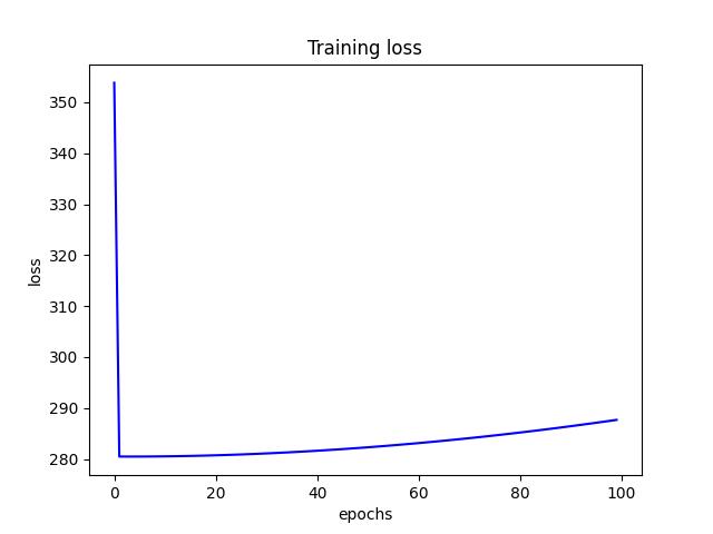
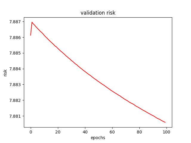
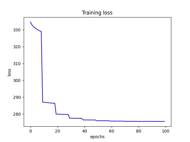
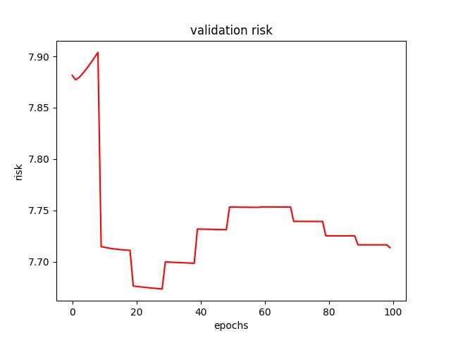
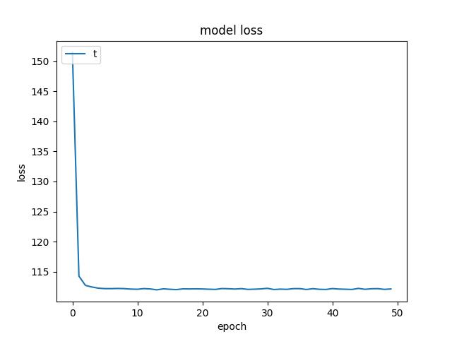
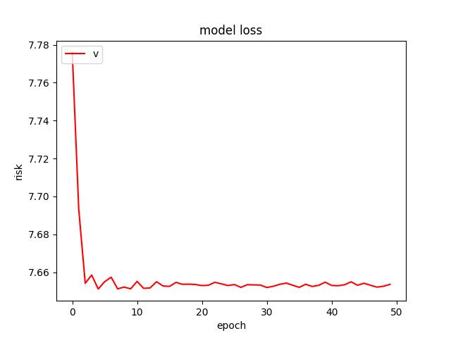
For L1 regularization, I found a learning rate (alpha) of 0.0001 and a $\lambda$ of 0.1 to produce the lowest test risk of 7.775. Below are a few figures from L1 tuning.

The learning curve of the validation MAE (alpha = 0.01, λ = 0.0001)

The learning curve of the training MSE (alpha = 0.0001, λ = 0.1)

The learning curve of the validation MAE (alpha = 0.0001, λ = 0.1)

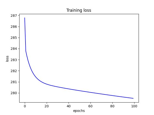
Figure 1.0: Learning curve of training and validation for L1 Regularization

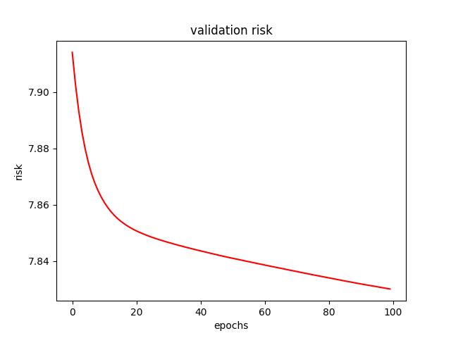
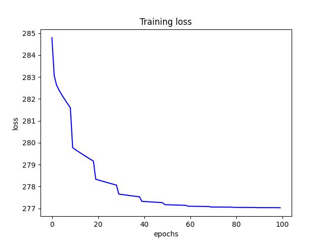
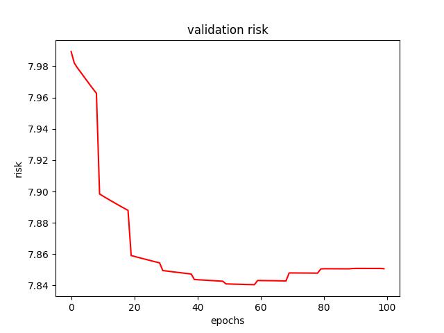
For L2 regularization, I found a learning rate of 0.0001 and a $\lambda$ of 0 (no L2 term) to produce the lowest test risk of 7.654087. Below are a few figures from L2 tuning.

The learning curve of the validation MAE (alpha = 0.001, λ = 0.1)

The learning curve of the training MSE (alpha = 0.1, λ = 0)

The learning curve of the validation MAE (alpha = 0.1, λ = 0)

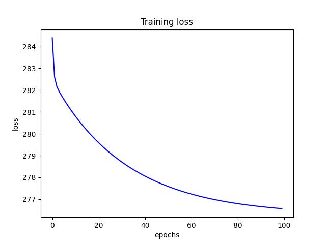
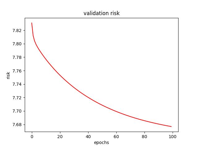
Figure 2.0: Learning curve of training and validation for L2 Regularization

Step Decay

I experimented with a few initial learning rates. After experimenting with different factors, I decided on a factor of 0.5 every 10 epochs. Thus every 10 epochs, the learning rate decreases by half.

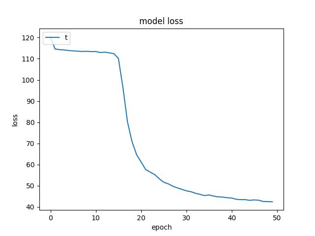
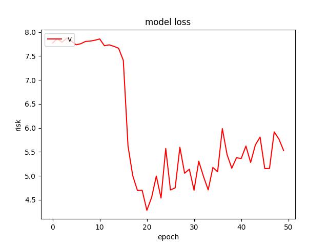
I found an initial learning rate (alpha) of 0.5 to produce the lowest test risk of 7.615133. Below are a few figures from decay tuning.

The learning curve of the training MSE (alpha = 0.5)

The learning curve of the validation MAE (alpha = 0.5)

The learning curve of the validation MAE (alpha = 0.1)

Figure 3.0: Learning curve of training and validation for learning rate step-decay

Neural Net Regression

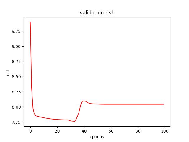
After tuning I found the best model to have a dropout layer of 0.3 and a RMSProp optimizer with He uniform weight initializer kernel. The lowest test risk it produced was 5.9898529052734375.

Optimizers

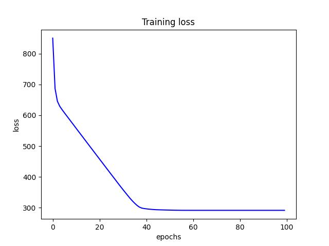
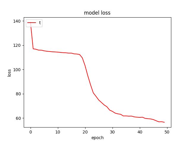
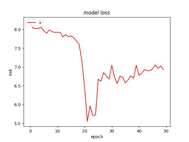
For an Adam optimizer with an initial learning rate of 0.01, I found a test risk of 7.744905948638916. Below are figures from Adam optimizer.
For an RMSProp optimizer (and He Uniform weight initializer kernel), I found the lowest test risk of 5.9898529052734375. Below are figures from RMSProp optimizer.

The learning curve of the training MSE (Adam optimizer)

The learning curve of the validation MAE (Adam optimizer)

Figure 4.0: Learning curve of training and validation for Adam optimzer (using a He uniform weight initializer kernel and a dropout of 0.3)

The learning curve of the training MSE (RMSProp optimizer)

The learning curve of the validation MAE (RMSProp optimizer)

Figure 5.0: Learning curve of training and validation for RMSProp optimzer (using a He uniform weight initializer kernel and a dropout of 0.3) 

Weight Initializer Kernels

For a normal, Gaussian weight initialization kernel, I found a test risk of 7.744905948638916. Below are learning curves.
For HE Uniform weight initialization kernel, I found the test risk of 5.9898529052734375. Figures can be found in figure 5.0 for He Uniform.

The learning curve of the training MSE (normal kernel)

The learning curve of the validation MAE (normal kernel)

Figure 6.0: Learning curve of training and validation for normal weight initializer kernel

Dropout

I found a dropout rate of 0.3 to produce the lowest test risk of . Figure for rate 0.3 can be found in figure 5.0. Below a few figures of tuning.

The learning curve of the validation MAE (dropout 0.6)

Figure 7.0: Learning curve of training and validation for dropout of 0.6

SVM Machine

I found a linear kernel to produce the lowest test risk of 7.778022035132583.

Conclusion

After experimenting with the three different machine learning models, I found using a neural network to produce the lowest risk I am able to get of 5.9898529052734375. I found the neural net to be the most memory intensive while the SVM was the least

References

R, Srivignesh. “A Walk-through of Regression Analysis Using Artificial Neural Networks in Tensorflow.” Analytics Vidhya, August 16, 2021, https://www.analyticsvidhya.com/blog/2021/08/a-walk-through-of-regression-analysis-using-artificial-neural-networks-in-tensorflow/.

“Training and evaluation with the built-in methods.” TensorFlow, Jan 10, 2022, https://www.tensorflow.org/guide/keras/train_and_evaluate.

“Machine Learning Models.” MathWorks, https://www.mathworks.com/discovery/machine-learning-models.

R, Srivignesh. “A Walk-through of Regression Analysis Using Artificial Neural Networks in Tensorflow.” Analytics Vidhya, March 27, 2021, https://www.analyticsvidhya.com/blog/2020/03/support-vector-regression-tutorial-for-machine-learning/.

Versloot, Christian. “How To Perform Multioutput Regression With Svms In Python.” Feb 15, 2022, https://github.com/christianversloot/machine-learning-articles/blob/main/how-to-perform-multioutput-regression-with-svms-in-python.m.

Code template of project.py from CMPUT 466

Code template of coding assignment 1 from CMPUT 466